Search Trees and Search Graphs
Unit 3: Search Techniques for Problem Solving — Section 3.2
You know how to formulate a search problem — states, actions, transition model, goal test, path cost. But formulation alone does not find solutions. This section explains the data structures that search algorithms actually use to explore state spaces, and a crucial decision every algorithm must make: should it remember where it has already been?
From States to Nodes
A state describes a configuration of the world. A node is a bookkeeping data structure that an algorithm builds while it explores.
- Node
-
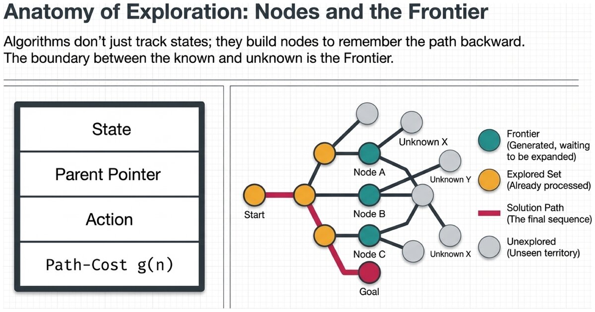
A data structure used during search that contains four fields: (1) state — the world configuration this node represents; (2) parent — the node that generated this one; (3) action — the action applied to the parent to reach this node; (4) path-cost — the total cost g(n) from the initial state to this node.
Why not just track states? Because to return a solution, the algorithm must reconstruct the sequence of actions that led to the goal. Nodes provide the chain of parent pointers needed to trace that path back to the start.
The Frontier
As a search algorithm runs, it expands nodes one at a time. Expansion means: apply every available action to generate all successor nodes, and add them to a waiting list.
- Frontier (Fringe)
-
The set of nodes that have been generated but not yet expanded. The frontier is the boundary between explored and unexplored territory. Different algorithms manage the frontier differently — a queue for BFS, a stack for DFS, a priority queue for UCS and A*.
The algorithm repeatedly picks a node from the frontier, checks whether it is the goal, and expands it if not. The critical question is: how does the algorithm pick the next node? That choice defines which algorithm you are running.
The Repeated-State Problem
Many state spaces contain multiple paths to the same state. In a city grid, you can reach intersection (2, 2) by going right then up, or up then right. Both paths lead to identical states, but a naive algorithm would treat them as separate nodes and expand each path separately.
A simple graph with redundant paths:
    A
   / \
  B   C
   \ /
    D
There are two paths from A to D: A → B → D and A → C → D. A search algorithm that ignores repeated states would expand D twice — once via B and once via C. In a large grid world, this redundancy can multiply into millions of wasted expansions.
Tree Search vs. Graph Search
The solution to repeated states is to remember which states have already been expanded. This creates two distinct approaches:
- Tree Search
-
Expands nodes without checking whether a state has been visited before. Simpler to implement and uses less memory, but may explore the same state many times. Can fail to terminate if the state space contains cycles.
- Graph Search
-
Maintains an explored set (also called the closed set) of states that have been expanded. Before expanding a node, graph search checks whether its state is already in the explored set. If so, it discards the node and moves on.
Graph-Search Algorithm (General):
-
Initialize the frontier with the root node (initial state, g = 0)
-
Initialize the explored set to empty
-
Loop:
-
If the frontier is empty, return failure
-
Remove a node from the frontier (choice determines the algorithm)
-
If the node’s state passes the goal test, return the solution (trace parent pointers)
-
Add the node’s state to the explored set
-
For each action available in the node’s state:
-
Generate the child node
-
If the child’s state is not in the frontier and not in the explored set, add it to the frontier
-
-
The addition of steps 2 and 5–6c is the entire difference between tree search and graph search. The code is slightly more complex, but the efficiency gain is often enormous.
When Does It Matter?
The practical impact of this choice depends on the state space structure.
Grid world navigation — 10×10 grid:
Tree search: Many redundant paths to each cell. The number of paths to a cell grows exponentially with distance from the start. Even a simple 10×10 grid can produce millions of nodes.
Graph search: Each cell is expanded at most once. Maximum nodes expanded: 100 (the size of the grid).
Graph search can be 1,000× or more faster for grid navigation.
The trade-off: graph search requires extra memory to store the explored set. When states are large or memory is extremely scarce, tree search with loop-detection may be preferred. For most practical problems, graph search is the right default.
When to prefer each approach:
Use tree search when the state space is genuinely a tree (no cycles, no redundant paths), or when memory is so scarce that the explored set is unaffordable.
Use graph search when the state space has cycles or redundant paths — which describes almost every realistic problem.
Summary of Key Structures
| Structure | Role |
|---|---|
Node |
Data structure storing state, parent, action, and path-cost |
Frontier |
The "to-do list" — generated but not yet expanded nodes |
Explored set |
Graph search only — states already expanded; prevents re-expansion |
Solution path |
Reconstructed by following parent pointers from the goal node back to the root |
Consider a map of your city modeled as a search graph.
-
What is a "state" in this problem?
-
Could you realistically reach the same intersection via two different routes?
-
How many times might a naive tree search expand a busy downtown intersection?
Now consider: what does this tell you about why real GPS applications use graph search?
Test your understanding of search structures and the tree vs. graph search distinction.
Based on the UC Berkeley CS 188 Online Textbook by Nikhil Sharma, Josh Hug, Jacky Liang, and Henry Zhu, licensed under CC BY-SA 4.0.
This work is licensed under CC BY-SA 4.0.