Evaluating Models
Unit 8: Machine Learning Foundations (Capstone) — Section 8.3
You now know how to train a decision tree and a k-NN classifier. But how do you know if your model is actually good? The answer is not simply "high accuracy on training data." A model that scores 99% on training data might be completely useless on new examples — it has memorized the training set rather than learning the underlying pattern. This section teaches you to evaluate models honestly and to diagnose the two failure modes: overfitting and underfitting.
See why models fail to generalize and how the bias-variance tradeoff explains it.
The Fundamental Challenge: Generalization
The goal of supervised learning is not to perform well on the training data you have seen — it is to perform well on new, unseen data that you will encounter in deployment.
The Student Analogy
-
Overfitting (memorizing): A student memorizes every practice problem and its exact answer. Gets 100% on practice tests but fails the real exam because the questions are slightly different. The student memorized answers, not concepts.
-
Underfitting (oversimplifying): A student decides to guess "C" for everything. Performs equally poorly on both practice tests and the real exam. They never engaged with the material.
-
Generalizing (just right): A student understands the underlying principles well enough to apply them to new problems. Performs well on both practice tests and the real exam.
Overfitting and Underfitting
Overfitting
Overfitting occurs when a model learns the training data too well — including its noise, errors, and coincidental patterns that do not reflect the true structure of the problem.
Signs of overfitting: * Training accuracy is very high (e.g., 99%) * Test accuracy is much lower (e.g., 65%) * The gap between training and test performance is large
- Overfitting
-
When a model is so closely fitted to the training data that it fails to generalize to new examples. An overfit model has memorized the training set rather than learned the underlying pattern. Symptom: high training accuracy, much lower test accuracy.
Underfitting
Underfitting occurs when a model is too simple to capture the patterns in the data. It performs poorly on both training and test data.
Signs of underfitting: * Training accuracy is low (e.g., 60%) * Test accuracy is similarly low (e.g., 58%) * The gap between training and test is small, but both scores are bad
- Underfitting
-
When a model is too simple to capture the underlying patterns in the data. An underfit model has not learned enough from training. Symptom: low accuracy on both training and test data.
The Bias-Variance Tradeoff
The concepts of overfitting and underfitting map onto a fundamental theoretical tension in machine learning: bias and variance.
- Bias
-
Error that arises when a model makes oversimplified assumptions about the data. High bias means the model misses real patterns (underfitting). Example: fitting a straight line to data that follows a curve.
- Variance
-
Error that arises when a model is too sensitive to the training data. High variance means the model captures noise as if it were signal (overfitting). Example: a decision tree that memorizes every training example.
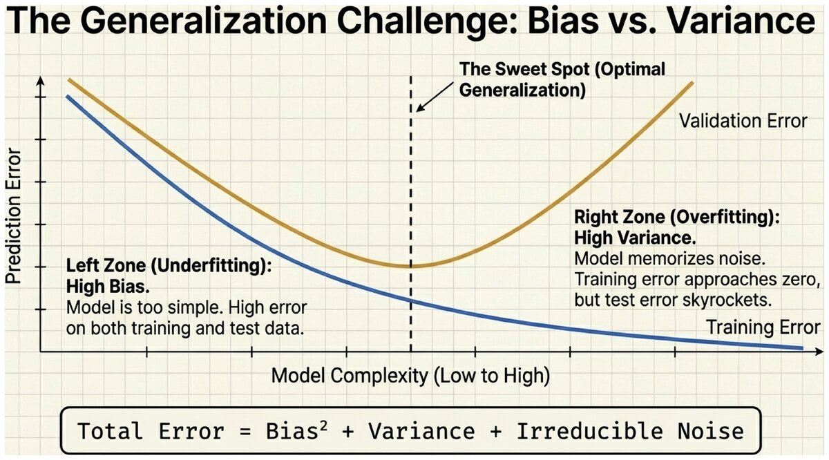
The Tradeoff: Reducing bias (making the model more complex) usually increases variance, and vice versa. The total prediction error is:
Total Error = Bias² + Variance + Irreducible Noise
The goal is to find the model complexity that minimizes the sum of bias and variance — not to minimize just one of them.
| Model | Bias | Variance |
|---|---|---|
Too simple (underfit) |
High — misses patterns |
Low — stable predictions |
Just right |
Low |
Low |
Too complex (overfit) |
Low |
High — sensitive to training noise |
Measuring Classification Performance
Before diagnosing overfitting, you need reliable metrics. Accuracy alone can be misleading, especially when one class is much more common than the other.
Accuracy
Accuracy is the simplest metric: the fraction of all predictions that are correct.
Accuracy
Accuracy = (Number of correct predictions) / (Total predictions)
If a model correctly classifies 143 out of 200 test examples, accuracy = 143/200 = 71.5%.
The Confusion Matrix
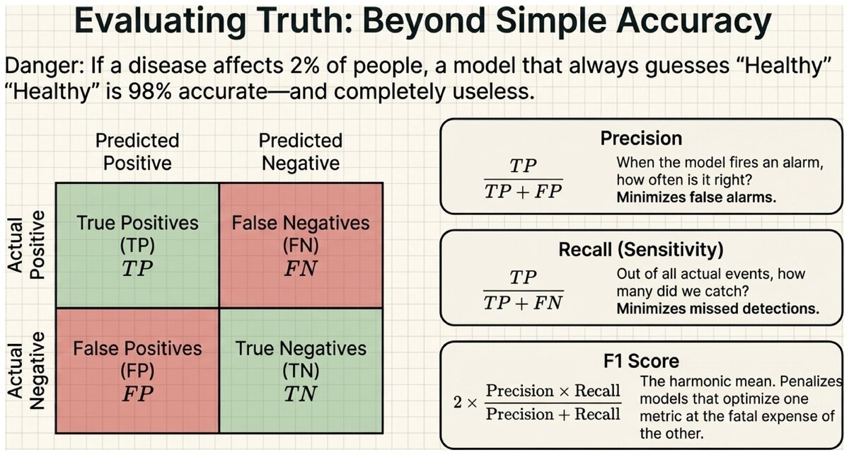
A confusion matrix shows all four possible outcomes for a binary classifier, not just overall accuracy.
| Predicted: Positive | Predicted: Negative | |
|---|---|---|
Actual: Positive |
True Positive (TP) — correctly predicted positive |
False Negative (FN) — missed a positive (Type II error) |
Actual: Negative |
False Positive (FP) — wrongly predicted positive (Type I error) |
True Negative (TN) — correctly predicted negative |
Precision
Precision answers: "Of all the times we predicted positive, how often were we right?"
Precision
Precision = TP / (TP + FP)
High precision means: when the model says "spam," it is usually correct. Low precision means: many legitimate emails are being flagged as spam (false alarms).
- Precision
-
The fraction of positive predictions that are actually correct. High precision indicates few false positives. Use precision when the cost of a false alarm is high (e.g., flagging a legitimate transaction as fraud).
Recall (Sensitivity)
Recall answers: "Of all the actual positives, how many did we catch?"
Recall
Recall = TP / (TP + FN)
High recall means: the model catches most real cases of the positive class. Low recall means: many actual positives are being missed.
- Recall (Sensitivity)
-
The fraction of actual positives that the model correctly identifies. High recall indicates few false negatives. Use recall when the cost of missing a real case is high (e.g., a cancer screening test that must catch every real cancer).
F1 Score
Precision and recall often trade off: making the model more cautious (predict positive only when very confident) increases precision but reduces recall. The F1 score is the harmonic mean of the two, rewarding models that balance both.
F1 Score
F1 = 2 × (Precision × Recall) / (Precision + Recall)
F1 ranges from 0 (worst) to 1 (perfect). A model with 100% precision and 0% recall has F1 = 0. A model with 67% precision and 60% recall has F1 ≈ 63%.
- F1 Score
-
The harmonic mean of precision and recall. Provides a single balanced metric that penalizes models that do well on one metric at the expense of the other. Particularly useful when classes are imbalanced.
Wine Quality Classifier Results (from the lab):
Suppose your decision tree (max_depth=5) produces these results on 200 test wines:
-
True Positives (good wine predicted as good): 46
-
True Negatives (normal wine predicted as normal): 102
-
False Positives (normal wine predicted as good): 21
-
False Negatives (good wine missed): 31
Calculations: * Accuracy: (46 + 102) / 200 = 74.0% * Precision: 46 / (46 + 21) = 68.7% * Recall: 46 / (46 + 31) = 59.7% * F1: 2 × (0.687 × 0.597) / (0.687 + 0.597) = 64.0%
Interpretation: The model is right about good wines most of the time when it says so (precision 69%), but it misses about 40% of actually good wines (recall 60%).
Techniques for Preventing Overfitting
Methods to Combat Overfitting:
-
Get more training data — more examples make it harder to memorize; best solution if available.
-
Cross-validation — split data into k equal folds; train on k-1 folds, test on the remaining fold; repeat k times. Produces a robust performance estimate without wasting data.
-
Regularization — add a penalty term to the training objective that discourages overly complex models.
-
Limit model complexity — set a maximum tree depth, use a larger k in k-NN.
-
Feature selection — remove irrelevant features that add noise without signal.
-
Ensemble methods — combine predictions from many models (e.g., Random Forests = many decision trees). Individual overfitting averages out.
- Cross-Validation
-
A model evaluation technique that divides the training data into k equal folds. The model is trained k times, each time using k-1 folds for training and 1 fold for validation. Final performance is the average across all k runs. Provides a more reliable performance estimate than a single train/test split.
Diagnosing Your Model
Reading the Training vs. Test Gap:
-
Small gap, both high: Your model is generalizing well. You are done.
-
Large gap (training >> test): Overfitting. Try limiting complexity (shallower tree, larger k), adding regularization, or getting more data.
-
Small gap, both low: Underfitting. Try a more complex model (deeper tree, smaller k), adding features, or using a different algorithm.
-
Test accuracy high but training lower: Very unusual; may indicate a bad train/test split. Check that splits were randomized.
The TensorFlow Playground (Apache 2.0) provides an interactive visualization of overfitting and the bias-variance tradeoff: playground.tensorflow.org
Adjust model complexity (layers, neurons) and watch how training vs. test error diverge as the model overfits.
Key Takeaways
Generalization — not training performance — is the ultimate test of a machine learning model. Accuracy alone can mislead; use precision, recall, and F1 to get a complete picture. The bias-variance tradeoff explains why more complex models are not always better: they fit the training data more closely but may fail on new examples. Diagnosing your model requires comparing training and test performance — a large gap signals overfitting, poor scores on both signals underfitting.
A medical screening test for a rare disease achieves 98% accuracy. Is that impressive?
-
The disease affects only 2% of the population.
-
A model that always predicts "no disease" would also score 98% accuracy.
-
Would you trust that model in a hospital?
What metric would you use instead, and why?
Practice evaluating classifiers using precision, recall, and F1.
Based on the UC Berkeley CS 188 Online Textbook by Nikhil Sharma, Josh Hug, Jacky Liang, and Henry Zhu, licensed under CC BY-SA 4.0.
Evaluation metrics adapted from scikit-learn Model Evaluation documentation, BSD License.
This work is licensed under CC BY-SA 4.0.