Comparing Search Algorithms

Unit 3: Search Techniques for Problem Solving — Section 3.6

You now have a toolkit of search algorithms. The question is no longer "how do these work?" but "which one should I use?" This section gives you the framework for answering that question systematically.

Four Performance Criteria

Every search algorithm can be evaluated along four dimensions. These criteria apply equally to uninformed and informed strategies.

Completeness: An algorithm is complete if it is guaranteed to find a solution whenever one exists. An incomplete algorithm may fail to terminate, loop forever, or report failure on solvable problems.
Optimality: An algorithm is optimal if it always returns a solution with the lowest possible path cost. A complete but non-optimal algorithm finds some solution, not necessarily the best one.
Time Complexity: The number of nodes generated (or expanded) as a function of the problem parameters. Expressed using b (branching factor), d (solution depth), m (max depth), and C* (optimal cost).
Space Complexity: The maximum number of nodes stored in memory at any point during the search. Often the practical bottleneck — a time-efficient algorithm that exceeds available memory cannot run.

The Complete Comparison Table

Algorithm	Complete	Optimal	Time	Space	Key Characteristic
BFS	Yes	Yes^a	O(b^d)	O(b^d)	Level-by-level expansion; memory-intensive
DFS	No^b	No	O(b^m)	O(b·m)	Explores one branch fully; memory-efficient
DLS	No^c	No	O(b^ℓ)	O(b·ℓ)	DFS bounded by a depth limit ℓ
ID-DFS	Yes	Yes^a	O(b^d)	O(b·d)	BFS completeness + DFS memory efficiency
UCS	Yes	Yes	O(b^⌈C*/ε⌉)	O(b^⌈C*/ε⌉)	Optimal for varying costs; no heuristic needed
Greedy	No^b	No	O(b^m)	O(b^m)	Fast; ignores path cost
A*	Yes	Yes^d	Exponential	Exponential	Optimal + efficient with admissible h(n)

Algorithm

Complete

Optimal

Time

Space

Key Characteristic

BFS

Yes

Yes^a

O(b^d)

Level-by-level expansion; memory-intensive

DFS

No^b

O(b^m)

O(b·m)

Explores one branch fully; memory-efficient

DLS

No^c

O(b^ℓ)

O(b·ℓ)

DFS bounded by a depth limit ℓ

ID-DFS

Yes

Yes^a

O(b^d)

O(b·d)

BFS completeness + DFS memory efficiency

UCS

Yes

O(b^⌈C*/ε⌉)

Optimal for varying costs; no heuristic needed

Greedy

No^b

O(b^m)

Fast; ignores path cost

Yes

Yes^d

Exponential

Optimal + efficient with admissible h(n)

^a Optimal only when all action costs are equal (finds shallowest, not cheapest, path).
^b Complete with graph search on finite spaces; can loop in infinite spaces.
^c Complete only if the solution is at depth ≤ ℓ.
^d Optimal when h(n) is admissible; graph search version requires h also be consistent.

Understanding Complexity with Real Numbers

Abstract complexity notation can be hard to interpret. Here is what these formulas mean concretely.

8-Puzzle performance comparison:

The 8-Puzzle has a branching factor of approximately b = 2.5 (average moves available) and typical solution depth d = 22.

Algorithm	Typical nodes expanded
BFS	~100,000
A* with misplaced tiles (h₁)	~10,000
A* with Manhattan distance (h₂)	~1,000
A* with pattern database	~100

Algorithm

Typical nodes expanded

BFS

~100,000

A* with misplaced tiles (h₁)

~10,000

A* with Manhattan distance (h₂)

~1,000

A* with pattern database

~100

Each improvement in heuristic quality produces roughly a 10× reduction in nodes expanded. A perfect heuristic (h = h*) would expand only the ~22 nodes on the optimal path.

BFS memory problem in practice:

If b = 10 and d = 12: * BFS frontier at depth 12: 10¹² = 1 trillion nodes * At 1,000 bytes per node: ~1 petabyte of memory * This is physically impossible on any standard machine

ID-DFS at the same depth: O(b·d) = 120 nodes in memory. That difference (10¹² vs. 120) illustrates why memory complexity matters as much as time complexity.

Algorithm Selection Guide

Choosing the right algorithm requires knowing three things about your problem:

Are action costs uniform or variable?
Do you have a good heuristic?
How much memory is available?

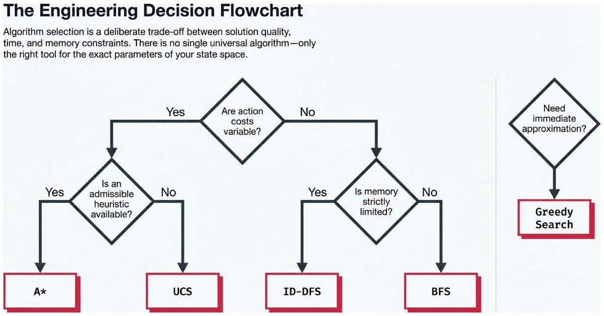
Decision flowchart for algorithm selection:

Do action costs vary?
- Yes → Use UCS or A* (if heuristic available)
- No → Continue to step 2
Is memory very limited?
- Yes → Use DFS (if any solution acceptable) or ID-DFS (if need optimal)
- No → Continue to step 3
Is an admissible heuristic available?
- Yes → Use A* (optimal + efficient)
- No → Use BFS (shallow solutions) or ID-DFS (large/deep spaces)

Situation	Recommended Algorithm
Shallow solutions, uniform costs, ample memory	BFS
Any solution acceptable, very limited memory	DFS
Large space, unknown depth, limited memory, uniform costs	ID-DFS
Variable costs, no heuristic	UCS
Good admissible heuristic available, optimality required	A*
Need a quick approximate answer, real-time constraint	Greedy best-first

Situation

Recommended Algorithm

Shallow solutions, uniform costs, ample memory

BFS

Any solution acceptable, very limited memory

DFS

Large space, unknown depth, limited memory, uniform costs

ID-DFS

Variable costs, no heuristic

UCS

Good admissible heuristic available, optimality required

Need a quick approximate answer, real-time constraint

Greedy best-first

Real-World Applications

GPS Navigation — A* with landmarks: Road networks have millions of intersections and variable edge weights (travel time). A* with a straight-line or preprocessed landmark heuristic finds optimal routes among millions of edges in milliseconds. The heuristic (straight-line distance to destination) is admissible because roads are never shorter than straight-line distance.

Robotics path planning — A* on a grid: A robot navigating a grid environment uses A* with Manhattan distance as the heuristic. The grid structure makes Manhattan distance admissible (robot moves horizontally and vertically). For high-dimensional configuration spaces, more sophisticated variants (RRT*, PRM*) extend these ideas.

Puzzle solving — IDA* with pattern databases: Solving the 15-puzzle or Rubik’s Cube optimally requires IDA* (iterative deepening A*) combined with precomputed pattern database heuristics. This approach solves problems in seconds that would take years with BFS.

Network routing — Dijkstra’s algorithm (≅ UCS): Internet routers use variants of UCS (commonly called Dijkstra’s algorithm in graph theory) to find shortest-path routes through the network. Link state routing protocols run UCS on each router’s local view of the network topology.

Practical Trade-Off Summary

No single algorithm is best for every problem. Each makes a deliberate trade-off:

BFS/ID-DFS: Choose correctness (completeness + optimality) over speed, with different memory profiles
DFS: Choose speed and memory over correctness — good when any solution suffices
UCS: Choose optimality without requiring a heuristic — pay the price in unexpanded nodes
A*: The best trade-off when a good heuristic exists — optimal, complete, and efficient; limited by memory
Greedy: Choose raw speed at the cost of optimality — useful when time matters more than solution quality

Understanding these trade-offs is not just academic. Every GPS app, robot, game AI, and automated planner chooses a search strategy based on exactly these considerations. The ability to reason about completeness, optimality, time, and space — and select accordingly — is a core skill in applied AI engineering.

Check your ability to select the appropriate algorithm for a given problem scenario.

Next: Lab — BFS on a Graph + A* on a Grid →

Based on the UC Berkeley CS 188 Online Textbook by Nikhil Sharma, Josh Hug, Jacky Liang, and Henry Zhu, licensed under CC BY-SA 4.0.

This work is licensed under CC BY-SA 4.0.