Supervised Learning Basics

Unit 8: Machine Learning Foundations (Capstone) — Section 8.2

You learned in Section 8.1 that supervised learning trains on labeled examples. But what does that look like in practice? This section walks through the full supervised learning workflow, introduces the two core problem types — classification and regression — and covers two foundational algorithms you will use in the lab: decision trees and k-Nearest Neighbors.

See the supervised learning framework in action.

Supervised Learning

Classification vs. Regression

Supervised learning divides into two types based on the kind of output we want to predict.

Classification

In a classification problem the output is a category selected from a fixed set of options.

Examples: * Email: spam or not spam (2 classes) * Image: cat, dog, or bird (3 classes) * Medical test: disease or healthy (2 classes) * Wine quality: good (≥ 6) or normal (< 6) — the lab task this week

Classification: A supervised learning problem in which the model predicts which discrete category an input belongs to. The output is a label from a fixed set (e.g., spam/not-spam, positive/negative, species name).

Regression

In a regression problem the output is a continuous numeric value anywhere on a scale.

Examples: * Predicted house price: $284,000 * Tomorrow’s temperature: 72.5°F * Student exam score: 87.3

Regression: A supervised learning problem in which the model predicts a continuous numeric value. Unlike classification, the output is not limited to a fixed set of categories.

The key distinction: classification asks "which bucket?" and regression asks "what number?" Use classification when your output is a label; use regression when your output is a measurement.

The Supervised Learning Workflow

All supervised learning projects follow the same seven-step pipeline, whether you are filtering spam or predicting stock prices.

Standard Supervised Learning Pipeline:

Collect and label data — Gather examples with correct answers. This is often the most time-consuming and expensive step.
Choose features — Decide which input variables (columns) to use. Better features produce better models.
Split data — Divide into a training set (the model learns from this) and a test set (used only to evaluate final performance). A common split is 80% training / 20% testing.
Choose algorithm — Select the learning algorithm: decision tree, k-NN, logistic regression, neural network, etc.
Train the model — Run the algorithm on training data. The model adjusts its internal parameters to minimize prediction error.
Evaluate on test set — Measure accuracy on examples the model has never seen. This is the true measure of how well the model generalizes.
Deploy and monitor — Use the model in production. Retrain periodically as new data arrives.

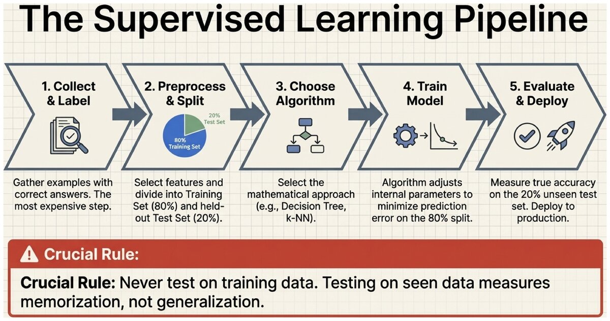
Never test on training data. Testing on training data is like giving students the exact exam questions during study time. The model will score perfectly on what it has already seen — but that tells you nothing about whether it can handle new situations. Always hold out a separate test set.

Decision Trees

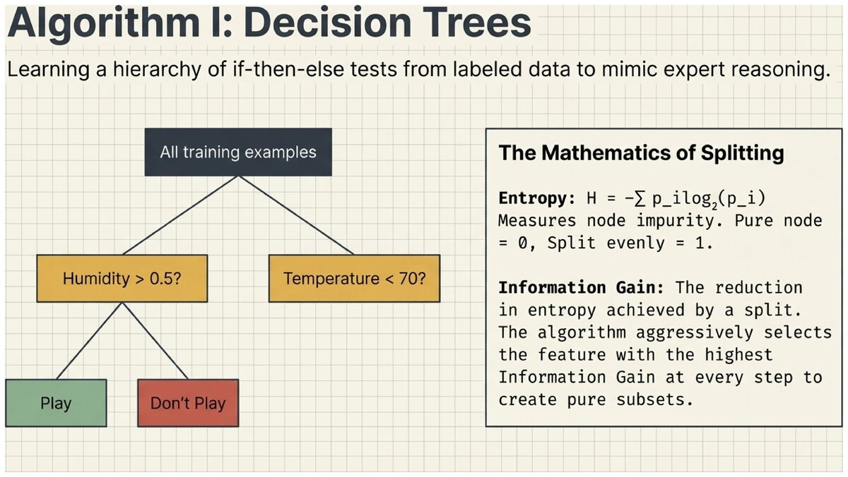
A decision tree is one of the most intuitive supervised learning algorithms. It learns a series of if-then-else questions from training data, organized into a tree structure that mimics how a human expert might make a decision.

See decision trees explained step by step.

Decision Trees Explained

Building a Decision Tree

Consider a doctor diagnosing a patient: "Does the patient have a fever? If yes, is there a cough? If yes with both, likely a respiratory infection." A decision tree automates this reasoning by learning which questions to ask and in what order from labeled training examples.

How the Decision Tree Algorithm Builds a Tree:

Start with all training examples at the root node.
Find the best feature to split on — the feature that most cleanly separates the classes. This is measured by information gain.
Split the data into subsets, one per value (or range) of that feature.
Recursively apply the same process to each child node.
Stop when all examples in a node belong to the same class, no more features remain, or a stopping condition (maximum depth, minimum samples) is met.

Information Gain and Entropy

How do we know which feature makes the "best" split? We want splits that create pure subsets — groups where one class dominates.

Entropy: A measure of impurity or uncertainty in a set of examples. A perfectly pure node (all one class) has entropy = 0. A node split evenly between two classes has maximum entropy = 1. Formula: H = -Σ p_i log₂(p_i), where p_i is the fraction of examples in class i.

Information Gain: The reduction in entropy achieved by splitting on a particular feature. We choose the feature with the highest information gain at each node — the feature that most reduces uncertainty about the class.

Decision Tree: Should I Play Tennis?

Suppose your training data includes weather observations labeled "play" or "don’t play." The algorithm might learn:

Outlook?
├── Overcast → Play (always!)
├── Sunny → Humidity?
│   ├── High → Don't Play
│   └── Normal → Play
└── Rain → Wind?
    ├── Strong → Don't Play
    └── Weak → Play

Each internal node is a question (a feature test). Each leaf node is a prediction (the class label). To classify a new day, you simply follow the branches from root to leaf.

Advantages and Limitations

Advantages	Limitations
Interpretable — you can read the tree and understand every decision	Overfitting — deep trees memorize training data (discussed in Section 8.3)
No preprocessing needed — handles both numerical and categorical features	Instability — small data changes can produce very different trees
Fast prediction — just traverse branches	Greedy — locally optimal splits may miss globally better trees
Non-linear — captures complex relationships	Biased toward dominant classes in imbalanced datasets

Advantages

Limitations

Interpretable — you can read the tree and understand every decision

Overfitting — deep trees memorize training data (discussed in Section 8.3)

No preprocessing needed — handles both numerical and categorical features

Instability — small data changes can produce very different trees

Fast prediction — just traverse branches

Greedy — locally optimal splits may miss globally better trees

Non-linear — captures complex relationships

Biased toward dominant classes in imbalanced datasets

Decision Tree: A supervised learning algorithm that learns a hierarchy of if-then-else tests (nodes) and class predictions (leaves) from labeled training data. Popular in regulated industries (finance, healthcare) because every prediction can be traced to an explicit chain of testable conditions.

K-Nearest Neighbors (k-NN)

K-Nearest Neighbors takes a completely different approach from decision trees. Instead of building a tree of rules, k-NN stores all training examples and classifies new data by looking at the most similar examples it has already seen.

The intuition: "Show me who your friends are, and I’ll tell you who you are." To classify a new wine, find the k wines in the training set that are most similar (based on chemical properties) and take a majority vote.

The k-NN Algorithm:

Store all training examples in memory (no model building occurs — k-NN is a lazy learner).
When a new example arrives, calculate the distance from that example to every training point.
Select the k nearest training examples (sorted by distance).
For classification: predict the majority class among the k neighbors.
For regression: predict the average value among the k neighbors.

Choosing k

The choice of k is the key hyperparameter in k-NN.

Effect of k on Predictions:

k = 1 — Classify based on only the single nearest neighbor. Very sensitive to noise and outliers. Tends to overfit.
k = 5 — Majority vote of 5 nearest neighbors. Smooths out local noise. A common starting point.
k = 50 — Considers a large neighborhood. Can underfit and lose local patterns.

Rule of thumb: try odd values (avoids ties) such as k = 3, 5, 7, 10, and use cross-validation to select the best k for your dataset.

K-Nearest Neighbors (k-NN): A supervised learning algorithm that classifies a new example by finding the k most similar training examples (by distance) and taking a majority vote. k-NN has no explicit training phase — it stores all data and computes distances at prediction time.

k-NN vs. Decision Trees

Aspect	Decision Tree	k-NN
Training time	Builds tree (moderate)	None — just stores data
Prediction time	Fast — follow branches	Slow — compute distances to all training points
Memory	Compact tree	Entire training set
Interpretability	High — explicit rules	Low — "nearby examples voted for this class"
New data	Must retrain	Add example to dataset immediately

Aspect

Decision Tree

k-NN

Training time

Builds tree (moderate)

None — just stores data

Prediction time

Fast — follow branches

Slow — compute distances to all training points

Memory

Compact tree

Entire training set

Interpretability

High — explicit rules

Low — "nearby examples voted for this class"

New data

Must retrain

Add example to dataset immediately

K-Nearest Neighbors is covered in depth in the supplementary page K-Nearest Neighbors (supplementary), including distance metrics (Euclidean, Manhattan), the curse of dimensionality, and practical guidance on feature scaling.

Key Takeaways

Supervised learning comes in two flavors — classification (predict a category) and regression (predict a number) — and follows a universal workflow: collect labeled data, split train/test, train an algorithm, and evaluate on held-out data. Decision trees learn explicit if-then rules that humans can read and verify. K-Nearest Neighbors classifies by similarity, with no explicit training phase. Both algorithms face the risk of overfitting, which is the subject of Section 8.3.

Test your understanding of the supervised learning concepts in this section.

Next: 8.3 Evaluating Models →

Based on the UC Berkeley CS 188 Online Textbook by Nikhil Sharma, Josh Hug, Jacky Liang, and Henry Zhu, licensed under CC BY-SA 4.0.

Code examples use scikit-learn, BSD License.

This work is licensed under CC BY-SA 4.0.