Introduction to Probabilistic Models

Unit 7: Probability and Uncertainty in AI — Section 7.5

Bayes' theorem is powerful for single-hypothesis reasoning, but real-world AI systems must reason about dozens or hundreds of variables simultaneously. A medical diagnosis system tracks symptoms, test results, patient history, and environmental factors. A self-driving car tracks road conditions, nearby vehicles, pedestrians, and traffic signals. How do we scale probabilistic reasoning to that complexity? This section introduces two practical answers: Bayesian networks (for structured probabilistic models) and naive Bayes classifiers (for fast, practical text classification).

Understand the core idea of Bayesian networks before reading.

Bayesian Networks Introduction

The Curse of Dimensionality

Consider building a full joint probability distribution for a medical system with 10 binary variables (symptoms and diseases):

2^10 = 1,024 probability values needed
With 20 variables: 2^20 = 1,048,576 values
With 30 variables: over 1 billion values

This exponential explosion makes full joint distributions impractical for any real system. Bayesian networks solve this problem by exploiting conditional independence to represent the same information compactly.

Bayesian Network: A directed acyclic graph (DAG) in which each node represents a random variable and each edge represents a direct probabilistic influence. Each node stores a conditional probability table (CPT) giving the probability of each value of the node given all combinations of its parents' values.

Structure of a Bayesian Network

A Bayesian network encodes a compact factorization of the full joint distribution. The key insight is that each variable is conditionally independent of its non-descendants given its parents.

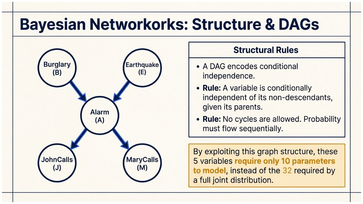
Simple Bayesian Network: Alarm

Classic BN with 5 nodes: Burglary (B), Earthquake (E), Alarm (A), JohnCalls (J), MaryCalls (M).

Burglary        Earthquake
    \          /
     v        v
      Alarm
     /    \
    v      v
JohnCalls  MaryCalls

Conditional probability tables:

P(B = true) = 0.001 (rare) P(E = true) = 0.002 (rare)

P(J=T | A=T) = 0.90, P(J=T | A=F) = 0.05 P(M=T | A=T) = 0.70, P(M=T | A=F) = 0.01

Total parameters: 1 + 1 + 4 + 2 + 2 = 10 numbers Without BN: 2^5 = 32 numbers needed for full joint distribution

The BN is more compact and encodes the causal structure: a burglary causes the alarm, the alarm causes John and Mary to call.

Conditional Probability Table (CPT): A table stored at each node of a Bayesian network that gives the probability of each possible value of the node for every combination of parent values. For a node with k binary parents, the CPT has 2^k rows.

Directed Acyclic Graph (DAG): A graph where edges have direction (arrows) and there are no cycles — you cannot follow arrows and return to where you started. Bayesian networks use DAGs because probability distributions over random variables must be consistent, and cycles would create circular dependencies that violate consistency.

Inference in Bayesian Networks

Once a Bayesian network is built, we use it to answer queries: given some observed evidence, what is the probability of some unobserved variable?

See how inference works in a Bayesian network step by step.

Bayesian Network Inference

There are two main types of inference:

Exact inference computes the exact posterior probability by summing over all unobserved variables. For small networks, this is computationally feasible. For larger networks, dynamic programming approaches like variable elimination make exact inference tractable.

Approximate inference uses sampling methods (like Monte Carlo sampling) to estimate probabilities when exact inference becomes too expensive.

Query: Given that JohnCalls and MaryCalls both called, what is P(Burglary)?

This is a diagnostic query — we observe the "symptoms" (calls) and want to infer the "cause" (burglary).

Query: P(Burglary = T | JohnCalls = T, MaryCalls = T)

The exact answer (computed by summing over Alarm and Earthquake) is approximately 0.284.

Without the Bayesian network and Bayes' theorem, there would be no principled way to compute this.

Causal vs. Diagnostic Reasoning

Bayesian networks support both directions of inference:

Causal (top-down): Given burglary, what is P(alarm sounds)?
Diagnostic (bottom-up): Given alarm sounded, what is P(burglary)?
Inter-causal: Given alarm sounded and no earthquake, what is P(burglary)? (Learning about one cause changes our belief about another — called "explaining away.")

Naive Bayes: A Practical Probabilistic Classifier

For text classification tasks — spam detection, sentiment analysis, topic categorization — a simplified version of Bayesian reasoning called naive Bayes is remarkably effective.

See naive Bayes applied to spam filtering with worked examples.

Naive Bayes and Spam Filtering

Naive Bayes Classifier: A probabilistic classifier that applies Bayes' theorem with a naive independence assumption: given the class label, all features are assumed to be conditionally independent of each other.

Despite this assumption being "naive" (almost never exactly true in real data), naive Bayes classifiers perform remarkably well in practice, especially for text classification.

The Naive Independence Assumption

For spam classification, the feature vector is the set of words in a message. A full Bayesian model would need to account for all correlations between words — "FREE" and "MONEY" tend to co-occur in spam. With a vocabulary of 10,000 words, the full joint likelihood table would be astronomically large.

Naive Bayes assumes that, given the class label (spam or ham), each word appears independently. This means:

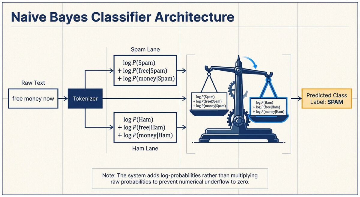
Naive Bayes Classification

P(Class | w₁, w₂, ..., wₙ) ∝ P(Class) × P(w₁ | Class) × P(w₂ | Class) × ... × P(wₙ | Class)

The "∝" means "proportional to" — we compute the unnormalized score for each class and pick the highest.

In practice, we use log probabilities to avoid numerical underflow:

log P(Class | words) ∝ log P(Class) + Σᵢ log P(wᵢ | Class)

Training a Naive Bayes Spam Filter

Building a Naive Bayes Classifier

Collect training data: a labeled dataset of spam and ham messages.

Compute prior probabilities:

P(Spam) = (# spam messages) / (# total messages)
P(Ham)  = (# ham messages)  / (# total messages)

Compute word likelihoods for each class:
```
P(word | Spam) = (# times word appears in spam + 1) / (# total words in spam + vocabulary size)
```
The "+1" is called Laplace smoothing — it prevents zero probabilities for words that never appeared in training.

Classify a new message:

score(Spam) = log P(Spam) + Σᵢ log P(wᵢ | Spam)
score(Ham)  = log P(Ham)  + Σᵢ log P(wᵢ | Ham)
Prediction  = argmax(score(Spam), score(Ham))

Mini Spam Filter: Manual Calculation

Training data: 6 messages total — 3 spam, 3 ham.

Spam messages contain: "free money win", "free prize claim", "win money now" Ham messages contain: "meeting tomorrow lunch", "project update report", "lunch tomorrow meeting"

Vocabulary size = 10 unique words.

Priors: P(Spam) = 3/6 = 0.50, P(Ham) = 3/6 = 0.50

Word likelihoods (with Laplace smoothing):

"free" in spam: appears 2/9 total spam words → (2+1)/(9+10) = 3/19 ≈ 0.158 "free" in ham: appears 0/9 total ham words → (0+1)/(9+10) = 1/19 ≈ 0.053

Classify new message: "free money"

score(Spam) = log(0.50) + log(3/19) + log(4/19)  [money appears 2× in spam: (2+1)/(9+10)]
           ≈ -0.693 + (-1.845) + (-1.556) = -4.094

score(Ham)  = log(0.50) + log(1/19) + log(1/19)  [money appears 0× in ham]
           ≈ -0.693 + (-2.944) + (-2.944) = -6.581

spam score (-4.094) > ham score (-6.581) → classified as SPAM. Correct!

Why Naive Bayes Works Despite Its Assumption

The naive independence assumption is almost certainly wrong — words in text are clearly correlated. Yet naive Bayes classifiers regularly achieve 95-99% accuracy on spam filtering tasks.

The explanation: for classification (picking the most probable class), we only need the ranking of classes to be correct, not the exact probability values. Even if the computed probabilities are wrong due to the independence assumption, the wrong probabilities often still rank the correct class highest.

This is a general principle in machine learning: a model that makes simplifying assumptions can still be highly useful if those simplifications do not disrupt the relative ordering of predictions.

Naive Bayes is simple, fast to train, fast to classify, and surprisingly effective. Its main weakness is that it cannot model feature interactions (e.g., "not free" is very different from "free," but a bag-of-words model treating negation like any other word misses this). For most text classification tasks, however, naive Bayes remains a strong baseline that more complex models must beat.

Summary Comparison: BN vs. Naive Bayes

Feature	Bayesian Network	Naive Bayes
Structure	Arbitrary DAG; captures causal relationships	Star topology: one class node, all features as children
Independence assumption	Conditional independence of non-descendants given parents	All features conditionally independent given class
Size of model	Can be very large; scales with causal complexity	Very compact: one prior per class, one CPT per word
Inference direction	Causal and diagnostic both supported	Diagnostic only (class given features)
Typical use	Medical diagnosis, robot localization, fault diagnosis	Text classification, spam filtering, sentiment analysis
Training data needed	Can be specified by experts or learned from data	Learned from labeled examples; works with small datasets

Feature

Bayesian Network

Naive Bayes

Structure

Arbitrary DAG; captures causal relationships

Star topology: one class node, all features as children

Independence assumption

Conditional independence of non-descendants given parents

All features conditionally independent given class

Size of model

Can be very large; scales with causal complexity

Very compact: one prior per class, one CPT per word

Inference direction

Causal and diagnostic both supported

Diagnostic only (class given features)

Typical use

Medical diagnosis, robot localization, fault diagnosis

Text classification, spam filtering, sentiment analysis

Training data needed

Can be specified by experts or learned from data

Learned from labeled examples; works with small datasets

Test your understanding of Bayesian networks and naive Bayes.

Next: Lab 7 — Spam Classifier →

Based on the UC Berkeley CS 188 Online Textbook by Nikhil Sharma, Josh Hug, Jacky Liang, and Henry Zhu, licensed under CC BY-SA 4.0.

This work is licensed under CC BY-SA 4.0.