Uninformed Search Strategies

Unit 3: Search Techniques for Problem Solving — Section 3.3

Imagine you’re trying to find a friend in a large building, but you have no idea which floor or room they’re in. One strategy: check every room on floor 1, then floor 2, then floor 3. Another strategy: go down the first hallway as far as it goes before trying any others. These two intuitions are the core of the two most fundamental search algorithms.

Uninformed Search: A family of search strategies that use only the information provided by the problem definition — initial state, actions, transition model, goal test, and path cost. Uninformed algorithms have no domain-specific knowledge about which states are "closer" to the goal. Also called blind search.

Four complexity terms appear repeatedly in this section. Commit them to memory:

b — branching factor: the average number of successors generated from each expanded node
d — depth of the shallowest solution in the search tree
m — maximum depth of the search tree (may be infinite)
ℓ — depth limit (for depth-limited search)

Breadth-First Search (BFS)

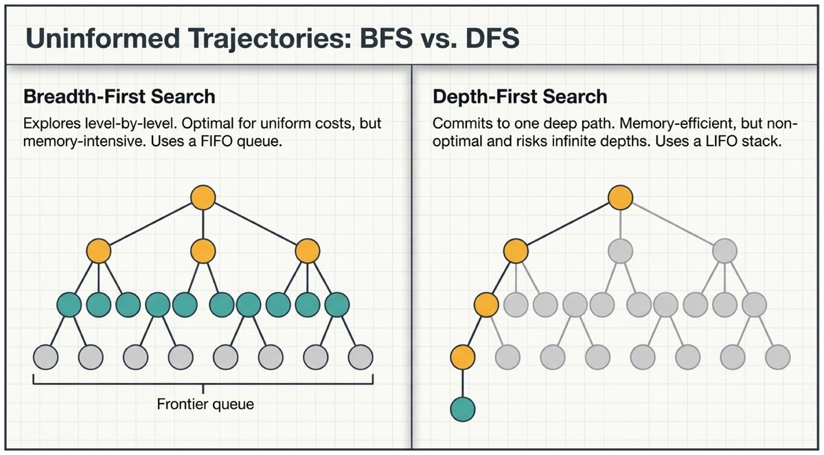
BFS expands the shallowest unexpanded node first — nodes are explored level by level, like ripples expanding from a pebble dropped in water.

Implementation: Use a FIFO queue (first-in, first-out) as the frontier.

BFS exploration order on a small tree:

         A (level 0)
        /|\
       B  C  D (level 1)
      /\  |
     E  F  G (level 2)

BFS explores: A, B, C, D, E, F, G All level-1 nodes are expanded before any level-2 node.

Property	Value	Explanation
Complete	Yes	BFS will find a solution if one exists, provided the branching factor b is finite.
Optimal	Yes*	BFS finds the shallowest goal. It is optimal only when all actions have the same cost.
Time complexity	O(b^d)	BFS must examine all nodes at depth d. If b=10 and d=12, that is 10¹² nodes — a trillion.
Space complexity	O(b^d)	The frontier holds all nodes at the current level. This is BFS’s main practical weakness.

Property

Value

Explanation

Complete

Yes

BFS will find a solution if one exists, provided the branching factor b is finite.

Optimal

Yes*

BFS finds the shallowest goal. It is optimal only when all actions have the same cost.

Time complexity

O(b^d)

BFS must examine all nodes at depth d. If b=10 and d=12, that is 10¹² nodes — a trillion.

Space complexity

O(b^d)

The frontier holds all nodes at the current level. This is BFS’s main practical weakness.

BFS’s Achilles' heel is memory, not time. The frontier at depth d stores O(b^d) nodes simultaneously. For b = 10 and d = 12, BFS needs roughly a trillion nodes in memory — far beyond any practical computer. BFS is excellent for problems with shallow solutions and small branching factors.

Depth-First Search (DFS)

DFS expands the deepest unexpanded node first — it commits to one path and follows it as deep as possible before backtracking.

Implementation: Use a LIFO stack (last-in, first-out) as the frontier.

DFS exploration order on the same tree:

         A (1)
        /|\
       B  C  D
      (2)(7)(8)
      /\  |
     E  F  G
    (3)(6)(9)

DFS explores: A, B, E, F, C, G, D It goes all the way down the leftmost branch before backtracking to siblings.

Property	Value	Explanation
Complete	No	DFS can get trapped in infinite loops (cycles). Graph search with an explored set fixes this.
Optimal	No	DFS returns the first solution found, which may be deep and expensive.
Time complexity	O(b^m)	Worst case: DFS explores the entire tree. If m is very large or infinite, this can be catastrophic.
Space complexity	O(b·m)	DFS only stores the current path plus unexplored siblings — far less than BFS.

Property

Value

Explanation

Complete

DFS can get trapped in infinite loops (cycles). Graph search with an explored set fixes this.

Optimal

DFS returns the first solution found, which may be deep and expensive.

Time complexity

O(b^m)

Worst case: DFS explores the entire tree. If m is very large or infinite, this can be catastrophic.

Space complexity

O(b·m)

DFS only stores the current path plus unexplored siblings — far less than BFS.

DFS’s advantage is memory efficiency. While BFS stores every node at the current depth level, DFS stores only the path from root to the current node plus its siblings. For b = 10 and m = 12, DFS needs ~120 nodes vs. BFS’s ~trillion. Use DFS when memory is scarce and you do not need the optimal solution.

Uniform-Cost Search (UCS)

BFS optimizes for depth (number of steps). But what if actions have different costs? A GPS cares about driving time, not the number of turns. UCS optimizes for total path cost.

Strategy: Always expand the node with the lowest path cost g(n).

Implementation: Use a priority queue ordered by g(n).

UCS on a weighted graph:

When choosing the next node to expand, UCS selects the cheapest cumulative cost. If the path A → C costs 2 and A → B costs 3, UCS expands C first, even though B is at the same depth.

This ensures that the first time the goal is reached, it has been reached via the cheapest path.

Property	Value	Explanation
Complete	Yes	Finds a solution if step costs are ≥ ε > 0 (prevents infinite zero-cost loops).
Optimal	Yes	Always finds the lowest-cost solution.
Time / Space	O(b^⌈C*/ε⌉)	C* is the optimal solution cost; ε is the minimum step cost.

Property

Value

Explanation

Complete

Yes

Finds a solution if step costs are ≥ ε > 0 (prevents infinite zero-cost loops).

Optimal

Yes

Always finds the lowest-cost solution.

Time / Space

O(b^⌈C*/ε⌉)

C* is the optimal solution cost; ε is the minimum step cost.

BFS is a special case of UCS. When all actions cost exactly 1, ordering by path cost g(n) is identical to ordering by depth. BFS and UCS produce the same results on uniform-cost problems; BFS is slightly faster because it uses a simpler queue.

Depth-Limited Search (DLS)

DFS’s incompleteness comes from diving into infinite paths. One fix: set a maximum depth and refuse to go deeper.

Strategy: Run DFS but treat nodes at depth ℓ as if they have no successors.

Property	Value	Explanation
Complete	No	Will miss solutions at depth > ℓ.
Optimal	No	Returns first solution found.
Time complexity	O(b^ℓ)	Bounded by depth limit ℓ.
Space complexity	O(b·ℓ)	Same as DFS, bounded by ℓ.

Property

Value

Explanation

Complete

Will miss solutions at depth > ℓ.

Optimal

Returns first solution found.

Time complexity

O(b^ℓ)

Bounded by depth limit ℓ.

Space complexity

O(b·ℓ)

Same as DFS, bounded by ℓ.

The obvious problem: choosing ℓ requires knowing the depth of the shallowest solution — information we usually do not have. If ℓ is too small, DLS misses the solution. If ℓ is too large, it wastes time on deep paths.

Iterative Deepening DFS (ID-DFS)

Iterative deepening solves the depth-limit problem elegantly: run DLS with ℓ = 0, then ℓ = 1, then ℓ = 2, and so on, stopping when a solution is found.

Iterative Deepening DFS:

Run DLS with depth limit ℓ = 0
If a solution is found, return it
Increment ℓ by 1
Repeat from step 1

Isn’t re-exploring shallow nodes on every iteration a terrible waste?

Actually no. In a tree with branching factor b = 10 and solution at depth d = 5:

Level 5 has ~100,000 nodes (10⁵)
Levels 0–4 together have ~11,111 nodes
ID-DFS re-explores levels 0–4 multiple times, but that total re-work adds less than 12% overhead

The extra work is small because most nodes live at the deepest level.

Property	Value	Explanation
Complete	Yes	Will eventually reach depth d if a solution exists.
Optimal	Yes*	Finds the shallowest solution (*when action costs are uniform).
Time complexity	O(b^d)	Same asymptotic bound as BFS.
Space complexity	O(b·d)	Like DFS — stores only the current path.

Property

Value

Explanation

Complete

Yes

Will eventually reach depth d if a solution exists.

Optimal

Yes*

Finds the shallowest solution (*when action costs are uniform).

Time complexity

O(b^d)

Same asymptotic bound as BFS.

Space complexity

O(b·d)

Like DFS — stores only the current path.

ID-DFS is usually the preferred uninformed search when the search space is large and solution depth is unknown. It achieves the completeness and optimality of BFS at the memory cost of DFS — the best of both worlds.

Comparing All Five Strategies

Algorithm	Complete	Optimal	Time	Space	Best Use Case
BFS	Yes	Yes*	O(b^d)	O(b^d)	Shallow solutions, ample memory, uniform costs
DFS	No	No	O(b^m)	O(b·m)	Deep solutions, very limited memory, any solution acceptable
DLS	No	No	O(b^ℓ)	O(b·ℓ)	Known depth bound
ID-DFS	Yes	Yes*	O(b^d)	O(b·d)	Large spaces, unknown depth, limited memory
UCS	Yes	Yes	O(b^⌈C*/ε⌉)	O(b^⌈C*/ε⌉)	Varying action costs, no heuristic available

Algorithm

Complete

Optimal

Time

Space

Best Use Case

BFS

Yes

Yes*

O(b^d)

Shallow solutions, ample memory, uniform costs

DFS

O(b^m)

O(b·m)

Deep solutions, very limited memory, any solution acceptable

DLS

O(b^ℓ)

O(b·ℓ)

Known depth bound

ID-DFS

Yes

Yes*

O(b^d)

O(b·d)

Large spaces, unknown depth, limited memory

UCS

Yes

O(b^⌈C*/ε⌉)

Varying action costs, no heuristic available

\*Optimal when all action costs are equal.

Explore BFS and DFS step-by-step with an interactive visualization at PathFinding.js (MIT License). Select "BFS" or "DFS" from the algorithm menu and watch how the frontier expands.

Check your understanding of uninformed search properties and algorithm selection.

Next: 3.4 Informed (Heuristic) Search →

Based on the UC Berkeley CS 188 Online Textbook by Nikhil Sharma, Josh Hug, Jacky Liang, and Henry Zhu, licensed under CC BY-SA 4.0.

This work is licensed under CC BY-SA 4.0.