Constraint Satisfaction Problems
Unit 4: Optimization and Constraint Satisfaction — Section 4.3
You are designing a university course schedule. Every class needs a time slot and a room. But two classes with the same instructor cannot overlap. A class cannot be assigned a room that is too small. Students taking required courses in sequence cannot face a conflict. There is no single "best" schedule in the optimization sense — any schedule that satisfies all these rules is a valid solution. This is a constraint satisfaction problem, and it calls for a fundamentally different approach than optimization.
What Is a Constraint Satisfaction Problem?
- Constraint Satisfaction Problem (CSP)
-
A problem defined by a set of variables, a domain of possible values for each variable, and a set of constraints that restrict which value combinations are permitted. The goal is to find an assignment of values to variables that satisfies all constraints.
A CSP has exactly three components:
-
Variables X = {X₁, X₂, …, Xₙ} — the decisions to be made
-
Domains D = {D₁, D₂, …, Dₙ} — the possible values for each variable (Xᵢ ∈ Dᵢ)
-
Constraints C = {C₁, C₂, …, Cₘ} — rules restricting which assignments are allowed
A solution is a complete assignment of values to all variables such that every constraint is satisfied.
Why CSPs Are Special
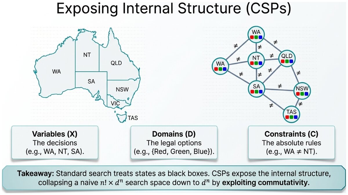
Standard search algorithms treat states as black boxes — they have no idea what structure lies inside. CSPs expose that structure explicitly.
| Aspect | Standard Search | CSP |
|---|---|---|
State |
Black box |
Defined by variable assignments |
Goal test |
Arbitrary function |
All constraints satisfied |
Successor function |
Arbitrary |
Assign a value to one unassigned variable |
Exploitation |
Problem-specific heuristics |
General-purpose constraint techniques |
Because assignments are commutative — assigning X=1 then Y=2 reaches the same state as Y=2 then X=1 — we never need to consider the order of assignments. This collapses the naive search space from n! × d^n to d^n, where n is the number of variables and d is the average domain size.
Classic Example: Australian Map Coloring
The map-coloring problem is the textbook introduction to CSPs. Color each territory of Australia so that no two adjacent territories share the same color.
Australian Map Coloring as a CSP:
Variables: {WA, NT, Q, NSW, V, SA, T} (Western Australia, Northern Territory, Queensland, New South Wales, Victoria, South Australia, Tasmania)
Domains: {Red, Green, Blue} for every variable
Constraints (adjacent territories must differ):
-
WA ≠ NT
-
WA ≠ SA
-
NT ≠ SA
-
NT ≠ Q
-
SA ≠ Q
-
SA ≠ NSW
-
SA ≠ V
-
Q ≠ NSW
-
NSW ≠ V
Note: Tasmania (T) is an island with no adjacency constraints — it can be any color.
One valid solution: WA=Red, NT=Green, Q=Red, NSW=Green, V=Red, SA=Blue, T=Red
The naive solution space contains 3^7 = 2,187 possible color assignments, but constraints eliminate the vast majority immediately.
The Constraint Graph
Binary constraints between pairs of variables can be represented visually as a constraint graph: nodes are variables, and an edge connects two variables when a constraint relates them.
- Constraint Graph
-
A graph where each node represents a CSP variable and each edge represents a binary constraint between two variables. The graph structure reveals independent subproblems and guides search heuristics.
The constraint graph reveals important structure. Tasmania’s isolated node tells us it can be solved independently. South Australia’s high degree (it borders six other territories) tells us it is the most critical variable to assign correctly — assigning it early and carefully will prevent many conflicts downstream.
Types of Constraints
Unary Constraints
A unary constraint restricts a single variable’s domain.
Example: X₁ ≠ Green (this territory may not be Green).
Unary constraints can always be handled by simply removing the disallowed values from the domain before search begins — they never require special search logic.
Binary Constraints
A binary constraint restricts a pair of variables.
Example: WA ≠ NT.
Binary constraints are the most common type and are directly represented in the constraint graph.
Global Constraints
A global constraint involves three or more variables, often all of them. The most common is all-different, which requires that a set of variables all receive distinct values.
- All-Different Constraint
-
A global constraint requiring that all variables in a specified set take distinct values. Used in Sudoku (all cells in a row, column, or box must have different values) and many scheduling problems.
Global constraints are more powerful than the equivalent collection of binary constraints. An all-different constraint on n variables encodes n(n-1)/2 pairwise inequality constraints in one compact rule, and specialized algorithms can enforce it much more efficiently than handling each pair separately.
Real-World CSP Examples
The N-Queens Problem
N-Queens as a CSP:
Variables: Q₁, Q₂, …, Qₙ — the queen in each column
Domains: {1, 2, …, n} — the row in which the queen is placed
Constraints (no two queens attack each other):
-
Row constraint: Qᵢ ≠ Qⱼ for all i ≠ j (no two queens in the same row)
-
Diagonal constraint: |Qᵢ − Qⱼ| ≠ |i − j| for all i ≠ j (no two queens on the same diagonal)
One 4-queens solution: Q₁=2, Q₂=4, Q₃=1, Q₄=3
By encoding the column position into the variable index, we automatically satisfy the column uniqueness requirement and reduce the domain from n² cells to n rows. Good problem formulation is a skill.
Sudoku
Sudoku as a CSP:
Variables: 81 cells, each indexed by (row, column)
Domains: * For pre-filled cells: domain = {given digit} * For empty cells: domain = {1, 2, 3, 4, 5, 6, 7, 8, 9}
Constraints: * All-different for each row (9 constraints) * All-different for each column (9 constraints) * All-different for each 3×3 box (9 constraints)
Total: 27 all-different constraints. A naïve solution space of 9^81 ≈ 2 × 10^77 becomes tractable because the constraints eliminate nearly all possibilities before the search even starts.
Class Scheduling
University Course Scheduling as a CSP:
Variables: One per course section to be scheduled
Domains: Set of (time slot, room) pairs
Constraints: * No instructor teaches two classes at the same time * Room capacity ≥ class enrollment * Classes required by the same students in the same semester don’t overlap * Instructor availability windows
This is the same type of problem a registrar solves every semester. CSP solvers can handle hundreds of courses with dozens of constraints automatically.
Cryptarithmetic
SEND + MORE = MONEY:
Assign a distinct digit (0–9) to each letter so that the arithmetic equation holds.
Variables: S, E, N, D, M, O, R, Y
Domains: {0, 1, 2, 3, 4, 5, 6, 7, 8, 9}
Constraints: * All-different (each letter gets a unique digit) * No leading zeros: S ≠ 0, M ≠ 0 * Arithmetic: the column equations with carry variables must hold
Solution: S=9, E=5, N=6, D=7, M=1, O=0, R=8, Y=2 Verification: 9567 + 1085 = 10652 ✓
Formulating a CSP: A Step-by-Step Process
Good CSP formulation is a design skill. The right formulation makes constraints simple and domains small.
How to Formulate a Problem as a CSP:
-
Identify variables — what are the decisions to make? Ask: "What do I need to assign a value to?"
-
Define domains — what values can each variable take? Start broad; constraints will narrow them.
-
Specify constraints — what rules must be satisfied? List every restriction on value combinations.
-
Check unary constraints — can any domains be immediately reduced? Remove impossible values from domains before search begins.
-
Draw the constraint graph — visualize which variables interact. High-degree nodes deserve early attention during search.
Consider the scheduling problem at your college. How would you formulate it as a CSP?
-
What are the variables? (Classes? Instructors? Rooms?)
-
What are the domains?
-
What constraints are hard requirements vs. preferences?
Notice that preferences ("this instructor prefers mornings") are soft constraints, while requirements ("no two classes in the same room at the same time") are hard constraints. Pure CSPs deal with hard constraints only. How might you handle soft constraints?
Why CSPs Are Tractable Despite Huge Search Spaces
The secret to CSP efficiency is that constraints let us detect dead ends before completing an assignment.
If WA = Red and NT must be assigned, we already know NT ≠ Red. We eliminate Red from NT’s domain immediately, reducing the choices we need to consider. If propagating this constraint causes another variable’s domain to become empty, we have detected a contradiction early — no need to finish the assignment just to find out it fails.
The power of the CSP framework comes from constraint propagation: using known assignments to reduce what remains possible for unassigned variables. Even before search begins, propagation can eliminate enormous portions of the solution space. The next two sections — 4.4 Backtracking Search and 4.5 Smart Heuristics — show how to harness this power systematically.
Constraint satisfaction problems provide a universal framework for problems where the goal is to find any valid configuration subject to a set of rules. Map coloring, Sudoku, scheduling, circuit design, and protein structure prediction all fit this mold. By making structure explicit — variables, domains, constraints — CSPs enable general-purpose algorithms that outperform hand-crafted search by orders of magnitude.
Practice formulating constraint satisfaction problems from natural language descriptions.
Based on the UC Berkeley CS 188 Online Textbook by Nikhil Sharma, Josh Hug, Jacky Liang, and Henry Zhu, licensed under CC BY-SA 4.0.
This work is licensed under CC BY-SA 4.0.