Local Search and Optimization
Unit 4: Optimization and Constraint Satisfaction — Section 4.1
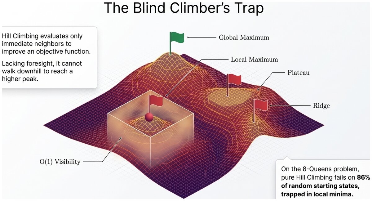
Imagine you are blindfolded on a mountain range, trying to reach the highest peak. You cannot see far, but you can feel the slope under your feet. Your instinct: always step uphill. That intuition is exactly how hill climbing works — and understanding when it succeeds and when it fails is the foundation of optimization in AI.
Discover why systematic search breaks down for large optimization problems, and how local search offers a practical alternative.
What Is Optimization?
An optimization problem asks you to find the best solution from a large set of possible configurations, where "best" is defined by a numerical score.
- Objective Function
-
A function f(state) that assigns a numerical value to every configuration in the search space. The goal is to find the state that maximizes (or minimizes) this value. Also called a fitness function, evaluation function, or cost function.
Unlike the search problems from Unit 3, optimization problems often have no clear "goal state" to reach — only a quality score to push as high (or low) as possible. The path to the solution rarely matters; only the final configuration counts.
Search vs. Optimization Compared:
| Aspect | Search (Unit 3) | Optimization (This Section) | |---|---|---| | Goal | Find any path to goal state | Find best configuration | | Success criterion | Reached goal state | Maximized/minimized objective | | Path matters? | Yes — sequence of actions | No — only final state | | Example | Route from A to B | Design best antenna shape |
The same problem can often be framed either way. Routing from city A to city B is search. Finding the shortest tour through 20 cities is optimization.
The Optimization Landscape
Visualize the state space as a terrain where the height at any point equals the objective function value. Finding the best solution means finding the highest peak.
- State Space Landscape
-
A conceptual visualization of an optimization problem where each point represents a possible configuration, and its height represents the objective function value. Optimization algorithms navigate this landscape.
Four important landscape features determine how hard a problem is to optimize:
-
Global maximum — the absolute highest point (the best solution)
-
Local maximum — a peak that is highest in its neighborhood, but not globally best
-
Plateau — a flat region where all neighboring states have the same value
-
Ridge — a narrow sequence of local maxima separated by downhill terrain
The challenge: most algorithms can only see their immediate neighborhood. They cannot tell a local maximum from the global one without exploring far more of the landscape.
The Hill Climbing Algorithm
Hill climbing is the simplest and most intuitive local search algorithm. It starts at a random state and repeatedly moves to the best neighboring state.
Hill Climbing:
-
Start at an initial state (often chosen randomly)
-
Generate all neighboring states (states reachable by one small change)
-
If the best neighbor is better than the current state, move there
-
Repeat until no neighbor is an improvement
-
Return the current state as the (local) optimum
The algorithm terminates when it reaches a local maximum — a state where every neighbor is equal or worse.
def hill_climbing(problem):
    current = problem.initial_state()
    while True:
        neighbors = problem.get_neighbors(current)
        best_neighbor = max(neighbors, key=problem.objective)
        if problem.objective(best_neighbor) <= problem.objective(current):
            return current   # local maximum reached
current = best_neighbor- Local Maximum
-
A state whose objective function value is greater than or equal to all of its neighbors. Hill climbing stops here even if a better state exists elsewhere in the landscape.
Algorithm Properties
Hill climbing has an extremely small memory footprint — it stores only the current state. This is both its greatest strength and its greatest limitation:
| Property | Hill Climbing |
|---|---|
Complete? |
No — can terminate at a local maximum, not the goal |
Optimal? |
No — returns the first local maximum it reaches |
Time complexity |
Highly landscape-dependent; typically fast in practice |
Space complexity |
O(1) — only the current state is stored |
The 8-Queens Problem: A Classic Example
The 8-queens problem asks you to place eight queens on an 8×8 chessboard so no two queens threaten each other.
Hill Climbing on 8-Queens:
-
State: A configuration of eight queens, one per column
-
Objective function: Number of attacking pairs (minimize — we want zero)
-
Neighbors: Move one queen to any other square in its column (56 neighbors per state)
-
Goal: Reach the state with zero attacking pairs
Performance: Hill climbing solves approximately 14% of random starting configurations outright. For the remaining 86%, it gets stuck at a local minimum where moving any single queen increases the number of attacks, yet the current configuration is not a solution.
Why does hill climbing fail on 86% of 8-queens starting states? A configuration can have zero pairs attacking in some region of the board, but adding or removing the last queen creates a new conflict. No single-step move improves things, so the algorithm declares it a local maximum — even though a valid solution exists just a few "wrong" moves away.
How might you help the algorithm escape this trap?
Three Pitfalls of Hill Climbing
Local Maxima
A local maximum looks like the top of the world from where the algorithm stands, but the global optimum lies somewhere else entirely. The algorithm has no mechanism to backtrack and explore alternative regions of the landscape.
Ridges
A ridge is a sequence of states that are locally optimal when moving perpendicular to the ridge, but can be improved by moving along it. Because hill climbing only tests immediate neighbors, it cannot "walk along" a ridge without first stepping downhill — which it refuses to do.
Plateaus
A plateau is a flat region where all neighbors have the same value. Hill climbing cannot determine which direction (if any) leads to higher ground. It may wander randomly for a long time, or declare the plateau edge a local maximum.
All three pitfalls — local maxima, ridges, and plateaus — arise from the same root cause: hill climbing commits fully to the best available neighbor without any memory or mechanism to escape suboptimal regions. Solutions to these pitfalls involve adding controlled randomness, not better gradient following.
Variants That Address the Pitfalls
Stochastic Hill Climbing
Instead of always choosing the single best uphill neighbor, stochastic hill climbing picks randomly from among all uphill moves. This makes it less likely to get trapped on narrow ridges, though it may converge more slowly.
First-Choice Hill Climbing
Generate neighbors one at a time, in random order, and move to the first one that is better than the current state. This is efficient when the branching factor is large — for 8-queens, there are 56 neighbors, so evaluating them all is wasteful. First-choice hill climbing finds an uphill move without examining the full neighborhood.
Random-Restart Hill Climbing
The most powerful and widely used variant. Run hill climbing from many different random starting states and return the best result found across all runs.
Random-Restart Hill Climbing:
-
Choose a random initial state
-
Run standard hill climbing to a local maximum
-
Record the result
-
Repeat steps 1–3 for a fixed number of restarts (or until time runs out)
-
Return the best local maximum found across all restarts
Performance on 8-Queens: Each run solves the problem with probability ~0.14. After k independent restarts, the probability of not finding a solution is (0.86)^k. With just 25 restarts, the chance of failing drops below 2%.
- Random Restart
-
A meta-heuristic that runs an optimization algorithm multiple times from different starting states to reduce the risk of getting trapped in a poor local optimum. With enough restarts, the algorithm is probabilistically complete.
When to Use Hill Climbing
Traveling Salesman Problem (TSP):
A salesperson must visit 20 cities and return home, minimizing total distance. With 20! ≈ 2.4 × 10^18 possible routes, systematic search is impossible.
Hill climbing approach: * State: An ordered list of cities (a tour) * Objective: Total distance (minimize) * Neighbors: Swap two cities in the tour
Random-restart hill climbing can find tours within a few percent of optimal in seconds — good enough for practical scheduling. The exact optimal tour would require exhaustive search that would take longer than the age of the universe.
Hill climbing is the right choice when:
-
The problem landscape is relatively smooth (few local maxima)
-
A "good enough" solution is acceptable
-
Memory is extremely limited (O(1) space)
-
You can afford multiple restarts from different starting points
-
The problem has a clear objective function and a well-defined neighborhood
It is a poor choice when:
-
You need a guaranteed optimal solution
-
The landscape is highly multimodal (many local maxima)
-
Each objective function evaluation is very expensive
Hill climbing is the computational equivalent of greedy improvement: fast, simple, and effective on smooth problems. Its failure on rugged landscapes motivates the more sophisticated algorithms in sections 4.2 through 4.6. Every improvement — simulated annealing, constraint propagation, smart heuristics — is essentially a way of escaping the trap that pure hill climbing falls into.
Test your understanding of local search and the hill climbing algorithm.
Based on the UC Berkeley CS 188 Online Textbook by Nikhil Sharma, Josh Hug, Jacky Liang, and Henry Zhu, licensed under CC BY-SA 4.0.
This work is licensed under CC BY-SA 4.0.