Simulated Annealing
Unit 4: Optimization and Constraint Satisfaction — Section 4.2
A blacksmith heats a piece of steel to glowing red, then cools it slowly. If cooled too fast, atoms freeze into a disordered structure full of defects. Cooled slowly, they settle into a perfect crystalline lattice — the lowest-energy, strongest arrangement. Simulated annealing borrows this physical process to escape the local-maximum trap that defeats hill climbing.
See how simulated annealing uses temperature to explore the optimization landscape more freely than hill climbing.
In Section 4.1, you saw that hill climbing gets stuck at local maxima because it never accepts a move that makes things worse. Simulated annealing fixes exactly this problem by sometimes accepting downhill moves — but with a probability that decreases as the algorithm runs.
The Metallurgy Inspiration
Physical annealing works in two phases:
-
Heating phase: Atoms absorb energy and move rapidly, breaking out of whatever structure they were locked into
-
Cooling phase: Atoms gradually lose energy and settle into lower-energy, more stable arrangements
-
Final state: If cooling is slow enough, atoms reach the global minimum-energy crystalline structure
The key insight: controlled randomness at high temperature allows the system to escape suboptimal configurations. As temperature drops, the system becomes increasingly conservative, refining whatever good structure it has found.
Simulated annealing maps this process to optimization:
-
Temperature controls the probability of accepting worse solutions
-
Energy corresponds to the objective function value
-
Cooling schedule gradually reduces temperature over time
The Simulated Annealing Algorithm
Simulated Annealing:
-
Start at an initial state with temperature T set to a high value
-
At each step, randomly select one neighbor of the current state
-
If the neighbor is better, move there (as in hill climbing)
-
If the neighbor is worse by an amount ΔE, move there anyway with probability e^(ΔE/T)
-
Decrease T according to the cooling schedule
-
Repeat until T reaches zero (or a minimum threshold)
-
Return the best state encountered
import math, random

def simulated_annealing(problem, schedule):
    current = problem.initial_state()
    best = current
    T = schedule.initial_temp

    for t in range(schedule.max_steps):
        T = schedule.temperature(t)
        if T == 0:
            return best
        neighbor = random.choice(problem.get_neighbors(current))
        delta_e = problem.objective(neighbor) - problem.objective(current)
        if delta_e > 0:
            current = neighbor          # better -- always accept
        elif random.random() < math.exp(delta_e / T):
            current = neighbor          # worse -- accept probabilistically
        if problem.objective(current) > problem.objective(best):
            best = current
return best- Simulated Annealing
-
A probabilistic local search algorithm that accepts worse solutions with probability e^(ΔE/T), where ΔE is the change in objective value and T is a temperature parameter that decreases over time. Named by analogy to the metallurgical annealing process.
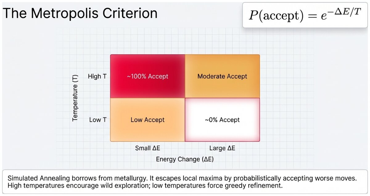
The Acceptance Probability
The mathematical heart of simulated annealing is the Metropolis criterion:
Acceptance Probability:
P(accept worse move) = e^(ΔE / T)
Where:
-
ΔE = objective(neighbor) − objective(current) < 0 (the neighbor is worse)
-
T = current temperature (positive)
-
e ≈ 2.718 (Euler’s number)
This formula has elegant behavior:
-
When T is high (early): e^(ΔE/T) ≈ 1 — almost any move is accepted, enabling broad exploration
-
When T is low (late): e^(ΔE/T) ≈ 0 — almost no worse moves are accepted; the algorithm behaves like hill climbing
-
When ΔE is small: More likely to accept (a slight degradation costs little)
-
When ΔE is large: Much less likely to accept (a large degradation is expensive)
Reading the acceptance probability:
Suppose the current solution has energy 100 and the neighbor has energy 103 (worse by ΔE = -3).
-
At temperature T = 10: P = e^(-3/10) = e^(-0.3) ≈ 0.74 — accept 74% of the time
-
At temperature T = 1: P = e^(-3/1) = e^(-3) ≈ 0.05 — accept only 5% of the time
-
At temperature T = 0.1: P = e^(-3/0.1) = e^(-30) ≈ 0.000000001 — essentially never
This graceful transition from exploration to exploitation is what makes SA effective.
Cooling Schedules
The cooling schedule determines how quickly T decreases and critically affects performance.
- Cooling Schedule
-
A function that specifies the temperature at each step of simulated annealing. The schedule must be slow enough to escape local optima but fast enough to be practical.
Three common schedules:
| Schedule | Formula | Characteristics | Typical Use |
|---|---|---|---|
Linear |
T(t) = T₀ − αt |
Simple; reaches zero quickly |
Small problems |
Exponential |
T(t) = T₀ × α^t |
Most common; α typically 0.85–0.99 |
General purpose |
Logarithmic |
T(t) = T₀ / log(1 + t) |
Very slow; guarantees convergence |
Theoretical benchmark |
In practice, exponential cooling is the standard choice. A cooling rate α between 0.95 and 0.99 provides enough time to explore while still converging in a reasonable number of steps.
If you set the cooling rate α = 0.999 (very slow cooling), simulated annealing will explore the landscape extensively but may take millions of steps. If you set α = 0.8 (fast cooling), it converges quickly but may miss better solutions.
How would you decide on a cooling rate for a new problem? What information would help you choose?
SA on the Traveling Salesman Problem
The Traveling Salesman Problem (TSP) is a canonical application for simulated annealing.
SA for TSP:
-
State: An ordered tour visiting all cities once
-
Neighbor: Reverse a random segment of the tour (2-opt swap)
-
Objective: Total tour distance (minimize — use negative distance for "energy")
Early phase (high temperature): SA accepts many bad swaps, exploring wildly across the solution space Middle phase (moderate temperature): SA occasionally accepts bad swaps, refining promising regions Late phase (low temperature): SA rarely accepts bad swaps, fine-tuning the best tour found
Result: SA routinely finds tours within 1–3% of optimal for hundreds of cities — solutions that would require astronomical computation to guarantee with systematic search.
Algorithm Properties
| Property | Simulated Annealing |
|---|---|
Complete? |
Yes, with logarithmic cooling (theoretical guarantee) |
Optimal? |
Approaches optimal with sufficiently slow cooling |
Time complexity |
Depends on cooling schedule; often O(max_steps) |
Space complexity |
O(1) — only current state and best state stored |
Best for |
Large spaces with many local optima |
The theoretical guarantee of SA — that logarithmic cooling converges to the global optimum — is mostly of academic interest. In practice, logarithmic cooling is too slow to be useful. The real value of SA is empirical: on many hard optimization problems, exponential cooling finds near-optimal solutions far faster than any alternative, including random-restart hill climbing.
A Brief Overview of Genetic Algorithms
Simulated annealing is not the only strategy for escaping local optima. Genetic algorithms (GAs) take a fundamentally different approach, maintaining an entire population of candidate solutions and combining them to produce better offspring.
- Genetic Algorithm
-
An optimization algorithm inspired by natural selection that maintains a population of candidate solutions and iteratively applies selection, crossover, and mutation operators to evolve better solutions.
The GA process each generation:
-
Selection: Choose the fittest individuals from the current population (they "reproduce")
-
Crossover: Combine two parent solutions to produce a child that inherits features from both
-
Mutation: Randomly alter one or more genes in a child solution (maintains diversity)
-
Replacement: New population of children replaces (or partially replaces) the old population
Genetic Algorithm for Binary Optimization:
If solutions are encoded as binary strings:
Parent 1: 1 1 0 0 1 1 0 0
Parent 2: 0 0 1 1 0 0 1 1
Single-point crossover at position 4:
Child: 1 1 0 0 0 0 1 1
A mutation might flip one bit:
Mutated: 1 1 0 0 0 1 1 1
GAs are powerful when solutions have a natural compositional structure — when good partial solutions can be meaningfully combined. They work well on problems with complex, multimodal landscapes where maintaining diversity across a population prevents premature convergence.
The trade-off: GAs require more configuration (population size, crossover rate, mutation rate) and more computational resources than SA, which only maintains a single solution at each step.
Comparing Local Search Techniques
| Technique | Explores how | Escapes local optima | Memory |
|---|---|---|---|
Hill Climbing |
Best neighbor |
No (random restart only) |
O(1) |
SA |
Random neighbor + probabilistic acceptance |
Yes (via temperature) |
O(1) |
Genetic Algorithm |
Population evolution + crossover |
Yes (via diversity) |
O(population size) |
Simulated annealing provides the best balance of simplicity and power among local search algorithms. It requires no more memory than hill climbing but can escape local optima through its temperature mechanism. For most single-solution optimization tasks, SA is the first algorithm to try beyond hill climbing. Genetic algorithms become compelling when solutions have natural building blocks that combine well, or when the problem naturally fits a population-based framing.
Test your understanding of simulated annealing and cooling schedules.
Based on the UC Berkeley CS 188 Online Textbook by Nikhil Sharma, Josh Hug, Jacky Liang, and Henry Zhu, licensed under CC BY-SA 4.0.
This work is licensed under CC BY-SA 4.0.